

Backtest metrics glossary: CAGR, MDD, Sharpe and Calmar ratios explained
What CAGR, real return, MDD, volatility, Sharpe, Sortino, Calmar and TWRR/MWRR measure, with example values, how Lifolio calculates them and common pitfalls.
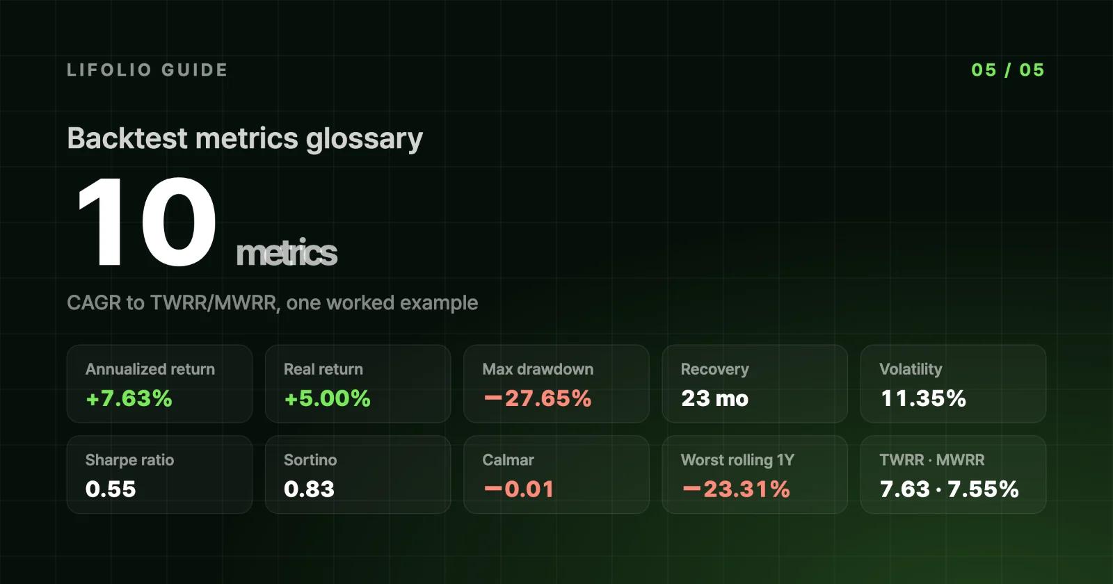
In this guide 11
The same results screen shows an annualized return of +7.63% alongside a Calmar ratio of −0.01. The mismatch comes from the first number covering all 10 years and the second only the last 3. This glossary walks through the ten metrics in Backtest results one by one: what each measures, how Lifolio calculates it, what it came to in the example, and where it's easy to misread.
The example is a US-dollar result for $10,000 in SPY 60% · TLT 40% from 2015-01-02 to 2024-12-31, rebalanced monthly. The full settings are in How to read backtest results.
| Metric | In one line | Example value |
|---|---|---|
| Annualized return (CAGR) | Total growth expressed as a constant yearly compound rate | +7.63% |
| Real return | Return after an assumed 2.5% annual inflation | +5.00% a year |
| Maximum drawdown (MDD) | Deepest drop from a peak | −27.65% daily · −26.21% month-end |
| Recovery time | From the bottom of the max drawdown back to the previous peak | 23 months |
| Volatility | How widely monthly returns swung (annualized) | 11.35% |
| Sharpe ratio | Excess return per unit of volatility | 0.55 |
| Sortino ratio | Excess return per unit of downside volatility | 0.83 |
| Calmar ratio | Trailing 36-month return ÷ max drawdown over the same window | −0.01 |
| Rolling returns | Same-length windows with different start dates | Worst 1-year holding period −23.31% |
| TWRR and MWRR | Performance of the investment vs performance of your money | 7.63% · 7.55% with $500 a month |
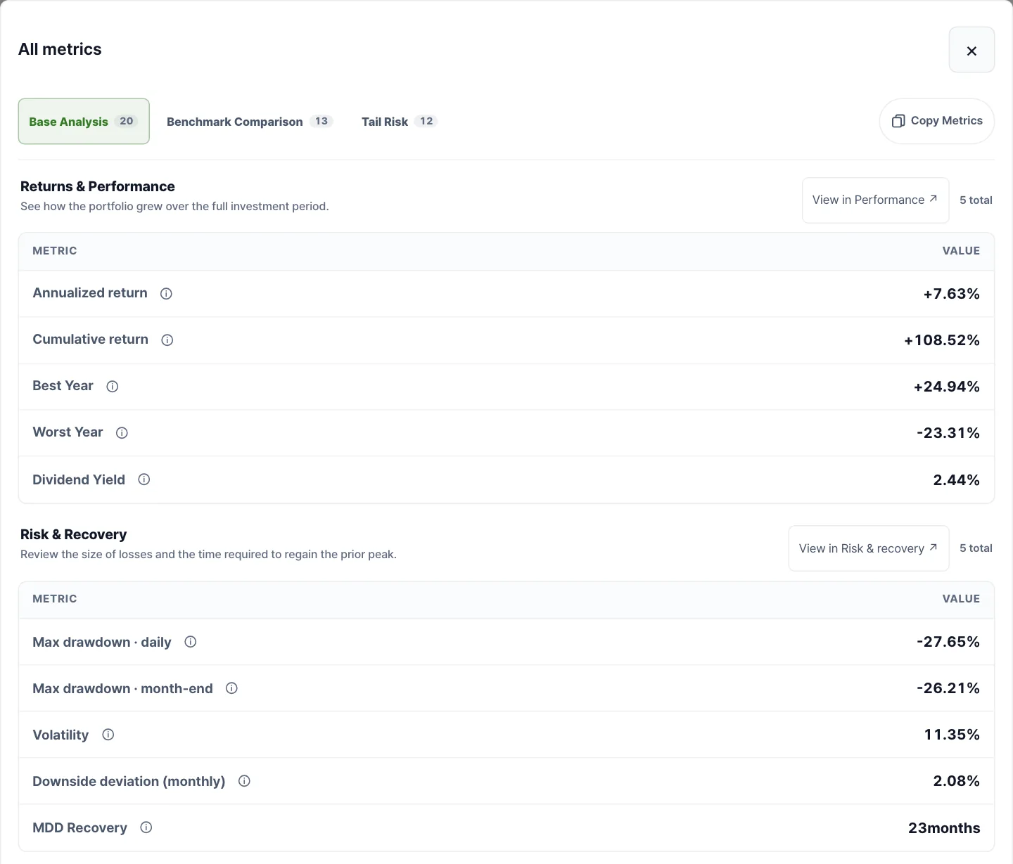
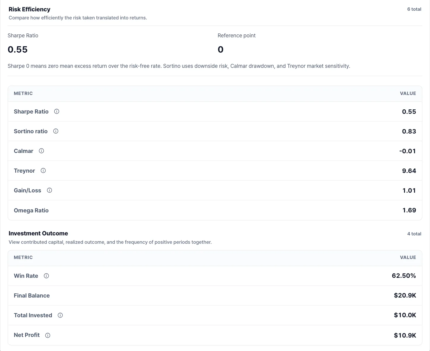
Open the All metrics window from the results screen and most of these metrics appear, grouped into four sections: Returns & Performance, Risk & Recovery, Risk Efficiency and Investment Outcome. The screenshots below show the first two sections, then the last two.
Annualized return (CAGR)
Over 10 years, $10,000 became $20,852. If it had grown at exactly the same rate every year, that rate would be 7.63%. That is the annualized return, or CAGR (compound annual growth rate). The summary card shows it as +7.6%.
Lifolio calculates it in two steps. First, for each day, it takes that day's value, subtracts any contribution made that day, and compares the result with the previous day's value to get a daily return. These daily returns are compounded through the end of the period to get the cumulative return. It then annualizes that with (1 + cumulative return)^(1 ÷ years) − 1. Chaining returns with contributions stripped out like this is the TWRR method described further down. If the period is shorter than a year, the cumulative return is shown as is, without annualizing.
The most common misconception is treating this figure as the average return you earned each year. A simple average of the example's ten annual returns is 8.54%, about 0.9 percentage points higher than the annualized figure. The more returns vary from year to year, the further the compound rate falls below the simple average.
Real return
Expand Purchasing power near the bottom of the Performance section and it turns a nominal annualized return of 7.63% into a real 5.00%, and a nominal cumulative return of 108.52% into a real 62.89%. Even while it is folded, its summary line reads "+5.0% a year after inflation · +7.6% before." The inflation removed here is not the actual consumer price index (CPI). It is a flat assumption that prices rise 2.5% every year, which is what "assuming 2.5% annual inflation" in the title refers to. The same 2.5% is used for won results.
The calculation divides rather than subtracts. The annualized figure is (1 + nominal annualized return) ÷ 1.025 − 1, and the cumulative figure is (1 + nominal cumulative return) ÷ 1.025^years − 1. That is why the result is 5.00%, slightly lower than the 5.13% you would get by simply subtracting 2.5 points from 7.63%.
It's easy to read this as adjusted for the actual inflation of those 10 years, but high-inflation and low-inflation years alike are calculated at 2.5%. Treat it as a reference figure that changes whenever the assumption does.
Maximum drawdown (MDD)
This is the largest percentage drop from the highest value reached so far. At each point in time, the value is divided by the highest value up to then, 1 is subtracted, and the lowest of those numbers is the MDD. Here too, the values have the effect of contributions removed. The −27.6% on the summary card is the daily figure, measured on every trading day. The All metrics window also shows the month-end figure, which uses only each month's last trading day.
MDD is the single largest drop that actually happened in this period, not a cap on the losses you might face in the future. When the two figures diverge sharply, and how to compare them with MDD from other services, are covered in MDD on a daily vs month-end basis, and recovery time.
Recovery time
This is how long it took to get from the bottom of the max drawdown back to the previous peak. In the example, the summary card shows it as "23 months from trough to recovery." Because it starts from the bottom rather than the peak, the total time spent below the peak is longer. If the peak hasn't been regained by the end of the period, "Recovering" appears instead of a number. How to read the down days and the recovery days separately is explained in MDD on a daily vs month-end basis, and recovery time.
Volatility (standard deviation)
This is how widely monthly returns were spread around their average, converted to an annual figure. Monthly returns are calculated from month-end values with the effect of contributions removed, excluding any partial month at the start or end of the period. The sample standard deviation of those returns is then multiplied by √12. The example comes to 11.35%.
This number ignores direction: a month with a big gain raises volatility just as much as a month with a big loss. A bigger caveat is that it captures only month-to-month swings. A decline that grinds lower a little at a time over several months barely registers, which is how this example, with volatility of 11.35%, still fell as much as −27.65% from its peak. There's a big gap between the intuition that "it moves about 11% a year" and the decline investors actually lived through.
Sharpe ratio
This measures how much return above the risk-free rate was earned per unit of volatility. For the definition, see The Sharpe Ratio, written by William F. Sharpe himself. Lifolio subtracts each month's risk-free rate from that month's return to get the excess return, divides the average excess return by its sample standard deviation, and multiplies by √12.
The risk-free rate depends on the reporting currency. Dollar results use the US 3-month Treasury bill rate, TB3MS (FRED), and won results use the 91-day CD rate from the Bank of Korea's ECOS. Each month uses the previous month's reading. The limits of using the CD rate as a risk-free rate are discussed in Why KRW returns differ from USD returns. If the required rate data is missing, metrics that depend on interest rates, such as the Sharpe ratio, are shown as N/A.
The example's Sharpe ratio is 0.55, and SPY's on the same settings is 0.76. When comparing with a Sharpe ratio from another source, check the inputs first. Whether it was calculated from daily or monthly returns, and what was used as the risk-free rate, can give the same portfolio different values.
Sortino ratio
The numerator is the same excess return as in the Sharpe ratio. Only the denominator changes, to downside deviation. Downside deviation squares only the negative parts of monthly excess returns, averages them, takes the square root and multiplies by √12. Every month counts in the average, with months at or above the threshold counted as a shortfall of zero.
The example comes to 0.83, higher than the Sharpe ratio of 0.55. Since the numerator is the same, this means swings on the downside were smaller than swings overall.
A common mistake is trying to recalculate the Sortino ratio from the Downside deviation (monthly) figure of 2.08% in the All metrics window. That figure uses 0%, not the risk-free rate, as its threshold, and it is a monthly value that hasn't been annualized. The formulas are different, so the numbers can't match.
Calmar ratio
This is the annualized return over the trailing 36 months divided by the month-end max drawdown (as an absolute value) over the same 36 months. Unlike the other metrics, which use the full period, it looks only at the latest 3 years. Yet the All metrics window labels it simply Calmar, and the 36-month detail appears only when you click the info icon next to the name, so it's easy to assume that, like the other numbers in the same table, it covers all 10 years.
In the example, the calculation window runs from January 2022 to December 2024, 36 monthly returns.
- Numerator: a balance of about $21,100 at the end of 2021 became $20,852 three years later. Annualized, that is −0.39%, the same as the 3-year value in the Trailing returns table in the Performance section.
- Denominator: the month-end max drawdown over the same window is −26.21%. The largest decline of the 10 years falls inside these 3 years, so the value is the same as the full period's month-end MDD.
- Ratio: −0.39 ÷ 26.21 ≈ −0.015, which the screen displays to two decimal places as −0.01.
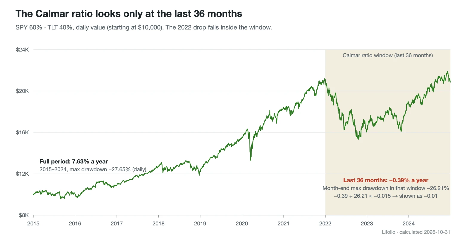
Divide the full period's annualized return by the full period's month-end MDD and you get about 0.29 (7.63 ÷ 26.21), so −0.01 is a number from an entirely different window. Because the window is always the last 3 years, moving the end date can swing the value a lot. End the same portfolio at the end of 2021 and the window shifts to 2019–2021, giving a Calmar ratio of 2.85. If there are fewer than 36 monthly returns, or no drawdown in that window, the ratio isn't calculated, and the full-period value isn't substituted either.
Rolling returns (holding-period outcomes)
Rolling returns measure many windows of the same length, changing only the start date. Holding-period outcomes in the Performance section slides an N-year window forward one month at a time, calculates the annualized return of each window, and for each holding period draws a bar from the worst result to the best, with the share of windows that ended in a loss beside it. Expand the table underneath to see the averages too. In the example there were 109 one-year windows, and the worst was January–December 2022, at −23.31%.
The windows overlap heavily, so the 109 can't be treated as 109 independent outcomes. The share of losing windows by holding period, and its limits, are covered in The limits of backtesting.
TWRR and MWRR (time-weighted and money-weighted returns)
Once you add or withdraw money along the way, there are two different ways to measure return. The time-weighted return (TWRR), as described under annualized return, chains returns with the effect of contributions stripped out, so it is the same no matter when or how much you put in. It shows the performance of the investment itself. The money-weighted return (MWRR) places the initial investment, each contribution and the final value on their actual dates and finds the discount rate at which their present values sum to zero: in other words, the internal rate of return (IRR). Periods when more money was invested carry more weight, so it comes closer to how your own money actually did. Lifolio groups cash flows by month for this calculation and reports the result as an annual rate.
MWRR is calculated only when the total invested is more than 1.01 times the initial investment, and in that case a Personal Return (MWRR) row appears in the All metrics window. If it differs from the summary card's annualized return by 0.05 percentage points or more, a "Counting when you added money" line is also added under the card. The default example, with no contributions, has no such line, and its 7.63% is the TWRR.
Put $10,000 into the same mix at the start and add $500 every month for 10 years, and the cards change like this.

Open the $500-a-month example in Lifolio
You put in $70,000 in total, and the final value is $108,684. The annualized return (TWRR) is 7.63%, exactly the same as without contributions, so the card still shows +7.6%. The MWRR, based on your own money, is 7.55%, shown on the card as "Counting when you added money: +7.5%". The max drawdown of −27.6%, the loss after a 1-year hold of 17% and the Sharpe ratio of 0.55 are also unchanged, because returns and risk metrics are all calculated with the effect of contributions removed.
The two differ by only 0.08 points because the same amount went in automatically every month. Money went in evenly in up and down months alike, so the luck of any single moment couldn't pull the result far. MWRR is very slightly lower, which can be read as the effect of having more money invested in the later years as contributions built up, while those last 3 years were weak at −0.39% a year.
The two diverge widely when a large sum goes in at one point in time. Invest a lump sum just before a downturn and that money takes the full hit, pushing MWRR below TWRR. Invest it just before a rebound and the opposite happens. TWRR stays the same either way, so the gap between the two numbers reflects when the money went in, not how the investment performed.
The full formulas and data-handling rules are in Methodology, and the sources of the interest-rate and exchange-rate data are in Data Sources. All values are calculated from historical data and do not predict future returns.
Frequently asked questions
What is a good Sharpe ratio?
There is no cutoff that holds in every case. Sharpe ratios are comparable only when the results share the same period, the same return frequency and the same risk-free rate. The example portfolio came to 0.55 for 2015–2024, but 1.18 when the backtest ended at the end of 2021. Rather than holding a single number up against a threshold, put it next to a benchmark calculated on the same settings (SPY's 0.76 in the example).
Is a negative Calmar ratio bad?
A negative value means the annualized return over the last 36 months was below zero. The example's −0.01 simply signals that a portfolio that returned 7.63% a year over the full 10 years went nowhere in the last 3. It isn't a verdict on the whole period. Be careful when comparing negative values, though. When the return is negative, a larger drawdown pushes the ratio closer to zero, so the portfolio that fell further can actually look better.
TWRR vs MWRR: which one should I use?
It depends on what you want to know. When comparing portfolios or strategies, TWRR, which strips out the effect of contribution amounts and timing, gives you a common yardstick. If you want to know what annual return the money you put in under your own contribution plan actually earned, look at MWRR. MWRR changes when contribution amounts and timing change, so to compare two portfolios' MWRR, you first need to give them identical contribution settings.
The numbers in this article were verified by rerunning the same settings on Nov 6, 2026. If you spot an error, please let us know using the Send Feedback button at the bottom right of the screen.